To create a chart in Excel for Mac, first select the data across a set of cells. Sometimes, you might not want to display all of your data. Choose the specific columns, rows, or cells that you want to include in the chart.
After you select your data, on the Insert tab, select Recommended Charts or choose a chart type directly from the Charts group.
Tip
Sometimes your data isn't arranged in Excel in a way that lets you create the type of chart you want. Learn how to arrange data for specific types of charts in Excel for Mac.
Select data from adjacent rows, columns, or cells
| To select | Here's what to do |
|---|---|
| Multiple adjacent columns | Position the cursor in the column header of the first column, and select while you drag to select adjacent columns. |
| Multiple adjacent rows | Position the cursor in the row header of the first row, and select while you drag to select adjacent rows. |
| Partial rows or columns | Position the cursor in the top left cell, and select while you drag to the bottom right cell. |
| All content in a table | Position the cursor anywhere in the table. |
| All content in a named range | Position the cursor anywhere in the named range. |
Select data from nonadjacent rows, columns, or cells
You can select specific rows, columns, or cells to include if your data isn't formatted as a table.
Tip
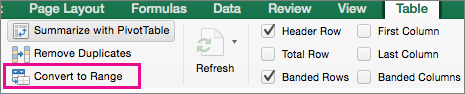
If your data is formatted as a table and you want to select nonadjacent information for a chart, first convert the table back to a normal range. Put the cursor in the table, and on the Table tab, select Convert to Range.
| To select | Here's what to do |
|---|---|
| Data in nonadjacent rows or columns | Position your cursor in the first row or column. Press COMMAND and select the other rows and columns you want. You can also do this by hiding the rows or columns in your worksheet. However, when you unhide the rows or columns, they automatically show up in the chart. |
| Data in nonadjacent cells | Position your cursor in the first cell. Press COMMAND and select the other cells you want. |
Select data from multiple worksheets
Create a summary worksheet to pull together data from multiple worksheets, and create the chart from the summary worksheet. To create the summary worksheet, copy data from each source worksheet, and then on the Paste menu, select Paste Link. By using Paste Link, when the data updates on your source worksheets, the summary worksheet and chart also update.
For example, if you have one worksheet for each month, you could make a 13th worksheet for the entire year that includes data from each of the monthly worksheets that you want for your chart.
Specify data ranges
Another way to create a chart is to select the type of chart you want, and then specify the data to include. You can also change the data range after you create a chart.
Note
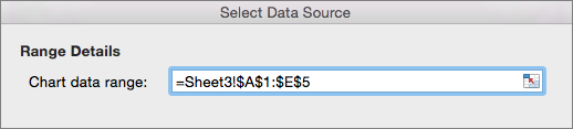
When you specify a chart data range in the Select Data dialog box, the selected range must be contiguous.
Follow these steps:
- On the Insert tab, select the chart type you want.
- On the Chart Design tab, select Select Data.

- Click in the Chart data range box, and then select the data in your worksheet.