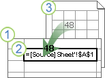
A workbook link (previously called an external reference) is a way to combine data from other workbooks or other sheets in the same workbook. You might want to use them to:
-
Link workbooks from several departments and then integrate pertinent data into a summary workbook. When the source workbooks change, the summary workbook is updated.
-
Create different views of data by creating several report workbooks that only link to pertinent data.
You can reference cells or a defined name in another workbook or the same workbook.
The workbook that contains the links is called the destination workbook, and the workbook that it's linked to is called the source workbook. You can link multiple source workbooks to a single destination workbook.
|
|
|
Method 1
-
Open the destination workbook that will contain the external reference and the source destination workbook that contains the data to which you want to create the workbook link.
-
Select the cell or cells where you want to create the external reference.
-
Type = (equal sign).
If you want to use a function, such as SUM, then type the function name followed by an opening parenthesis. For example, =SUM(.
-
Switch to the source workbook, and then click the worksheet that contains the cells that you want to link.
-
Select the cell or cells that you want to link to and press Enter.
Note: If you select multiple cells, like =[SourceWorkbook.xlsx]Sheet1!$A$1:$A$10, and have a current version of Microsoft 365, then you can simply press ENTER to confirm the formula as a dynamic array formula. Otherwise, the formula must be entered as a legacy array formula by pressing CTRL+SHIFT+ENTER. For more information on array formulas, see Guidelines and examples of array formulas.
-
Excel will return you to the destination workbook and display the values from the source workbook.
-
Note that Excel will return the link with absolute references, so if you want to copy the formula to other cells, you'll need to remove the dollar ($) signs:
=[SourceWorkbook.xlsx]Sheet1!$A$1
If you close the source workbook, Excel will automatically append the file path to the formula:
='C:\Reports\[SourceWorkbook.xlsx]Sheet1'!$A$1
Method 2
-
Open the destination workbook that will contain the workbook link and the source workbook that contains the data that you want to link to.
-
In the source workbook, select the cell or cells you want to link.
-
Press Ctrl+C or go to Home > Clipboard > Copy.
-
Switch to the destination workbook, and then click the worksheet where you want the linked data to be placed.
-
Select the cell where you want to place the linked data, and select Home > Clipboard > Paste > Paste Link.
-
Excel returns the data you copied from the source workbook. If you change it, it will automatically change in the destination workbook.
-
Open the destination workbook that will contain the external reference and the source workbook that contains the data to which you want to create the workbook link.
-
Select the cell or cells where you want to create the external reference.
-
Type = (equal sign).
-
Switch to the source workbook, and then click the worksheet that contains the cells that you want to link.
-
Press F3, select the name that you want to link to and press Enter.
Note: If the named range references multiple cells, and you have a current version of Microsoft 365, then you can simply press ENTER to confirm the formula as a dynamic array formula. Otherwise, the formula must be entered as a legacy array formula by pressing CTRL+SHIFT+ENTER. For more information on array formulas, see Guidelines and examples of array formulas.
-
Excel will return you to the destination workbook and display the values from the named range in the source workbook.
-
Open the destination workbook and the source workbook.
-
In the destination workbook, select Formulas > Defined Names > Define Name.
-
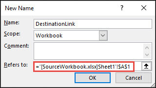
In the New Name dialog box, in the Name box, type a name for the range.
-
In the Refers to box, delete the contents, and then keep the cursor in the box.
If you want the name to use a function, enter the function name, and then position the cursor where you want the external reference. For example, type =SUM(), and then position the cursor between the parentheses.
-
Switch to the source workbook, and then click the worksheet that contains the cells that you want to link.
-
Select the cell or range of cells that you want to link, and click OK.
There are different ways Formulas with workbook links are displayed.
When the source workbook is open, the workbook link in the destination workbook includes the workbook name in square brackets ([ ]), followed by the worksheet name, an exclamation point (!), and the cells that the formula depends on. For example:
=SUM([Budget.xlsx]Annual!C10:C25)
When the source workbook is not open, the workbook link in the destination workbook includes the entire path. For example:
=SUM('C:\Reports\[Budget.xlsx]Annual'!C10:C25)
Note: If the name of the other worksheet or workbook contains spaces or non-alphabetical characters, you must enclose the name (or the path) within single quotation marks as in the example above. Excel will automatically add these for you when you select the source range.
Formulas that link to a defined name in another workbook use the workbook name followed by an exclamation point (!) and the defined name. For example:
=SUM(Budget.xlsx!Sales)
When you create a workbook link, both workbooks must be saved in an online location you can reach with your Microsoft 365 account.
Important: Workbook links are considered potentially unsafe and must be enabled when you open a formula workbook. When you open a formula workbook, click Enable Content in the Message Bar to allow the workbook links to function. If you don't, Excel keeps the most recent values and disables refreshing the links with values from the data workbook.
Method 1
-
Open the destination workbook that will contain the external reference and the source destination workbook that contains the data to which you want to create the workbook link.
-
Select the cell or cells where you want to create the external reference.
-
Type = (equal sign).
If you want to use a function, such as SUM, then type the function name followed by an opening parenthesis. For example, =SUM(.
-
Switch to the source workbook, and then click the worksheet that contains the cells that you want to link.
-
Select the cell or cells that you want to link to and press Enter.
Note: If you select multiple cells, like =[SourceWorkbook.xlsx]Sheet1!$A$1:$A$10, and have a current version of Microsoft 365, then you can simply press ENTER to confirm the formula as a dynamic array formula. Otherwise, the formula must be entered as a legacy array formula by pressing CTRL+SHIFT+ENTER. For more information on array formulas, see Guidelines and examples of array formulas.
-
Excel saves the formula in the destination workbook but cannot change the tab back to the destination workbook.
-
Note that Excel will return the link with absolute references, so if you want to copy the formula to other cells, you'll need to remove the dollar ($) signs. Full cloud file path is used in the URL:
=SUM('https://microsoft-my.sharepoint.com/personal/v-mathavale_microsoft_com/Documents/[data.xlsx]Sheet1'!$A$6:$A$9)
Method 2
-
Open the destination workbook that will contain the workbook link and the source workbook that contains the data that you want to link to.
-
In the source workbook, select the cell or cells you want to link.
-
Press Ctrl+C or go to Home > Clipboard > Copy.
-
Switch to the destination workbook, and then click the worksheet where you want the linked data to be placed.
-
Select the cell where you want to place the linked data, and select Home > Clipboard > Paste > Paste Link.
-
Excel returns the data you copied from the source workbook. If you change it, it will automatically change in the destination workbook when you refresh your browser window.
See Also
Define and use names in formulas
Description of workbook link management and storage in Excel


