When you create an Excel table, a table Header Row is automatically added as the first row of the table, but you have to option to turn it off or on.
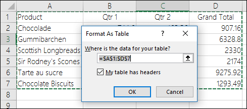
When you first create a table, you have the option of using your own first row of data as a header row by checking the My table has headers option:
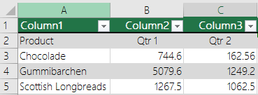
If you choose not to use your own headers, Excel will add default header names, like Column1, Column2 and so on, but you can change those at any time. Be aware that if you have a header row in your data, but choose not to use it, Excel will treat that row as data. In the following example, you would need to delete row 2 and rename the default headers, otherwise Excel will mistakenly see it as part of your data.

Notes:
-
The table header row should not be confused with worksheet column headings or the headers for printed pages. For more information, see Print rows with column headers on top of every page.
-
When you turn the header row off, AutoFilter is turned off and any applied filters are removed from the table.
-
When you add a new column when table headers are not displayed, the name of the new table header cannot be determined by a series fill that is based on the value of the table header that is directly adjacent to the left of the new column. This only works when table headers are displayed. Instead, a default table header is added that you can change when you display table headers.
-
Although it is possible to refer to table headers that are turned off in formulas, you cannot refer to them by selecting them. References in tables to a hidden table header return zero (0) values, but they remain unchanged and return the table header values when the table header is displayed again. All other worksheet references (such as A1 or RC style references) to the table header are adjusted when the table header is turned off and may cause formulas to return unexpected results.
Show or hide the Header Row
-
Click anywhere in the table.
-
Go to Table Design on the Ribbon.
-
In the Table Style Options group, select the Header Row check box to hide or display the table headers.
-
If you rename the header rows and then turn off the header row, the original values you input will be retained if you turn the header row back on.
Notes:
-
The table header row should not be confused with worksheet column headings or the headers for printed pages. For more information, see Print rows with column headers on top of every page.
-
When you turn the header row off, AutoFilter is turned off and any applied filters are removed from the table.
-
When you add a new column when table headers are not displayed, the name of the new table header cannot be determined by a series fill that is based on the value of the table header that is directly adjacent to the left of the new column. This only works when table headers are displayed. Instead, a default table header is added that you can change when you display table headers.
-
Although it is possible to refer to table headers that are turned off in formulas, you cannot refer to them by selecting them. References in tables to a hidden table header return zero (0) values, but they remain unchanged and return the table header values when the table header is displayed again. All other worksheet references (such as A1 or RC style references) to the table header are adjusted when the table header is turned off and may cause formulas to return unexpected results.
Show or hide the Header Row
-
Click anywhere in the table.
-
Go to the Table tab on the Ribbon.
-
Select the Header Row check box to hide or display the table headers.
-
If you rename the header rows and then turn off the header row, the original values you input will be retained if you turn the header row back on.
Show or hide the Header Row
-
Click anywhere in the table.
-
Select the Table Design tab > Table Style Options > Header Row.
Need more help?
You can always ask an expert in the Excel Tech Community or get support in Communities.
See Also
Create or delete an Excel table
Resize a table by adding or removing rows and columns
Filter data in a range or table


