Excel help & learning

Analyze, understand, and visualize your data with ease
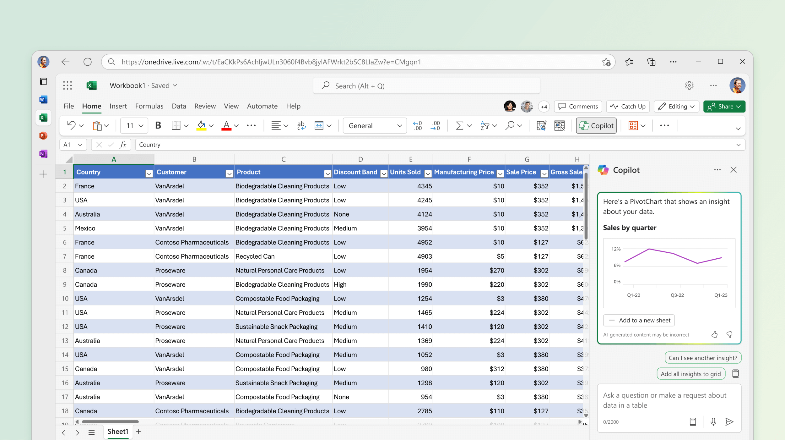
Copilot in Excel helps you generate formulas, analyze and summarize data, and add helpful visuals to spreadsheets.
Get started with Copilot in Excel
Identify insights with Copilot in Excel
Generate formulas with Copilot in Excel
Get AI-powered features in Microsoft 365
Explore Excel

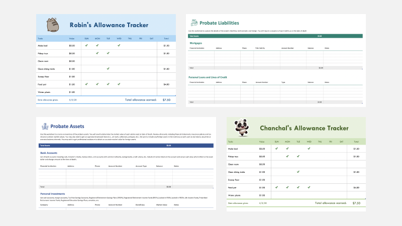
Find Excel templates
Bring your ideas to life and streamline your work by starting with professionally designed, fully customizable templates from Microsoft Create.
Find customizable templates to take your project to the next level

Analyze Data
Ask questions about your data without having to write complicated formulas. Not available in all locales.
Use Analyze Data to make data analysis simpler, faster, and more intuitive

Are you a small business?
Visit the small business help & learning page to learn how you can use Microsoft 365 in your small business.
Explore ways to help your small business grow, finish projects faster, and do more

Support for Excel 2016 and Excel 2019 has ended
Learn what end of support means and how to upgrade to Microsoft 365.
Get details about the end of support for Office 2016 and Office 2019
Trending topics
Customize your data
Follow your stocks
Use linked data types to track and analyze stock data. Or analyze trends based on geographical locales.

