The XMATCH function searches for a specified item in an array or range of cells, and then returns the item's relative position.
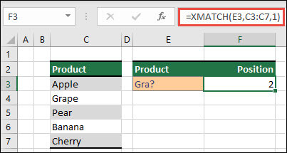
Assume we have a list of products in cells C3 through C7 and we wish to determine where in the list the product from cell E3 is located. Here, we'll use XMATCH to determine an item's position within a list.
Syntax
The XMATCH function returns the relative position of an item in an array or range of cells.
=XMATCH(lookup_value, lookup_array, [match_mode], [search_mode])
|
Argument |
Description |
|---|---|
|
lookup_value Required |
The lookup value |
|
lookup_array Required |
The array or range to search |
|
[match_mode] Optional |
Specify the match type: 0 - Exact match (default) -1 - Exact match or next smallest item 1 - Exact match or next largest item 2 - A wildcard match where *, ?, and ~ have special meaning. |
|
[search_mode] Optional |
Specify the search type: 1 - Search first-to-last (default) -1 - Search last-to-first (reverse search). 2 - Perform a binary search that relies on lookup_array being sorted in ascending order. If not sorted, invalid results will be returned. -2 - Perform a binary search that relies on lookup_array being sorted in descending order. If not sorted, invalid results will be returned. |
Examples
Example 1
The exact position of the first phrase that exactly matches or comes closest to the value of "Gra" is determined in the example that follow.
Formula: XMATCH(E3,C3:C7,1)
Example 2
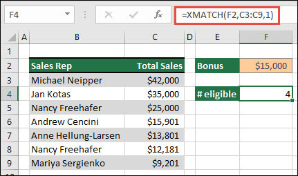
The number of salespeople qualified for a bonus is determined in the following example. In order to discover the closest item in the list or an exact match, this also uses 1 for the match_mode; however, because the data is numeric, it returns a count of values. Since there were four sales representatives that exceeded the bonus amount in this instance, the function yields 4.
Formula=XMATCH(F2,C3:C9,1)
Example 3
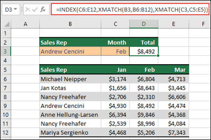
Next, we'll perform a simultaneous vertical and horizontal lookup using a mix of INDEX/XMATCH/XMATCH. In this instance, we would want the sales total for a certain sales representative and month to be returned. This is comparable to combining INDEX and MATCH methods, but it takes less arguments.
Formula=INDEX(C6:E12,XMATCH(B3,B6:B12),XMATCH(C3,C5:E5))
Example 4
In addition, XMATCH can be used to return a value within an array. =XMATCH(4,{5,4,3,2,1}), for instance, would provide 2 because 4 is the array's second entry. While =XMATCH(4.5,{5,4,3,2,1},1) produces 1 in this exact match case, the match_mode argument (1) is configured to return either an exact match or the next largest item, which is 5.
Need more help?
You can always ask an expert in the Excel Tech Community or get support in Communities.


