In a chart you create, axis labels are shown below the horizontal (category, or "X") axis, next to the vertical (value, or "Y") axis, and next to the depth axis (in a 3-D chart). Your chart uses text from its source data for these axis labels.
The techniques shown here are performed in Excel. If you're using Word, PowerPoint, or Outlook, when you insert a chart, Excel is opened to edit your data. These changes can then be done in Excel and apply when you return to your other app.
Don't confuse the horizontal axis labels—Qtr 1, Qtr 2, Qtr 3, and Qtr 4, as shown below, with the legend labels below them—East Asia Sales 2009 and East Asia Sales 2010.
Change the text of the axis labels
-
Select each cell in the worksheet that contains the label text you want to change.
-
Type the text you want in each cell, and press Enter.
As you change the text in the cells, the labels in the chart are updated.
Make label text that's different from the worksheet labels
(This procedure only works in Excel) To keep the text in the source data on the worksheet the way it is, and just create custom labels in the chart, you can enter new label text that's independent of the worksheet data:
-
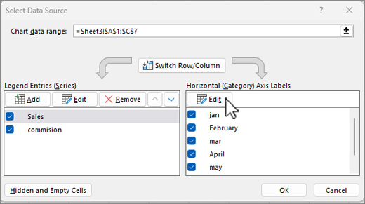
Right-click the category labels you want to change, and choose Select Data.
-
In the Horizontal (Category) Axis Labels box, select Edit.
-
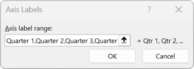
In the Axis label range box, enter the labels you want to use, separated by commas.
For example, type Quarter 1,Quarter 2,Quarter 3,Quarter 4.
Change the format of text and numbers in labels
To change the format of text in category axis labels:
-
Right-click the category axis labels you want to format, and select Font.
-
On the Font tab, choose the formatting options you want.
-
On the Character Spacing tab, choose the spacing options you want.
To change the format of numbers on the value axis:
-
Right-click the value axis labels you want to format.
-
Select Format Axis.
-
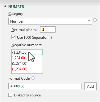
In the Format Axis pane, select Number.
Tip: If you don't see the Number section in the pane, make sure you've selected a value axis (it's on the left).
-
Choose the number format options you want.
If the number format you choose uses decimal places, you can specify them in the Decimal places box.
-
To keep numbers linked to the worksheet cells, check the Linked to source box.
Note: Before you format numbers as percentages, make sure that the numbers shown on the chart have been calculated as percentages in the worksheet, or are shown in decimal format like 0.1. To calculate percentages on the worksheet, divide the amount by the total. For example, if you enter =10/100 and format the result 0.1 as a percentage, the number is correctly shown as 10%.
Tip: An axis label is different from an axis title, which you can add to describe what's shown on the axis. Axis titles are not automatically shown in a chart. To add them, see Add or remove titles in a chart.


