When you create a PivotTable or PivotChart, Excel assigns default names to each of these objects by using the following naming conventions: PivotTable1, PivotTable2, and so on; and Chart 1, Chart 2, and so on. However, you can change the name of each object to make it more meaningful to you.
Rename a PivotTable
-
Click the PivotTable.
-
Go to PivotTable Tools > Analyze, and in the PivotTable group, click the PivotTable Name text box.
-
Type a new name.
-
Press ENTER.
Rename a PivotChart
-
Click the PivotChart.
-
Go to PivotChart Tools > Analyze tab, in the PivotChart group, click the Chart Name text box.
-
Type a new name.
-
Press ENTER.
Rename a PivotTable
-
Click the PivotTable.
-
In the PivotTable Analyze ribbon tab, click the PivotTable Name text box.
-
Type a new name.
-
Press ENTER.
PivotTable on iPad is available to customers running Excel on iPad version 2.82.205.0 and above. To access this feature, please ensure your app is updated to the latest version through the App Store.
Rename a PivotTable
1. Tap anywhere in the PivotTable to show to the PivotTable tab on the ribbon.
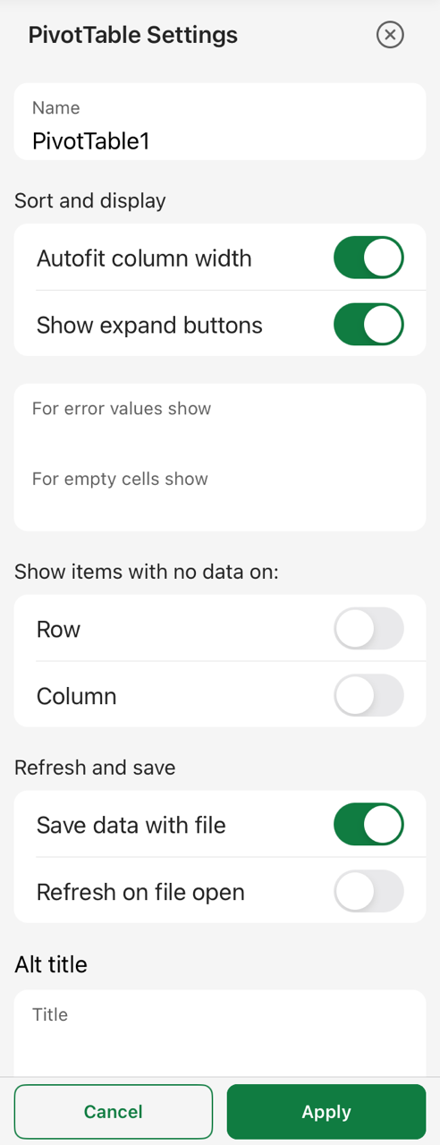
2. Tap Settings to display the PivotTable Settings side pane.
3. In the Name box, type a new name.
4. Tap Apply.
Need more help?
You can always ask an expert in the Excel Tech Community or get support in Communities.


