Date tables in Power Pivot are essential for browsing and calculating data over time. This article provides a thorough understanding of date tables and how you can create them in Power Pivot. In particular, this article describes:
-
Why a date table is important for browsing and calculating data by dates and time.
-
How to use Power Pivot to add a date table to the Data Model.
-
How to create new date columns such as Year, Month, and Period in a date table.
-
How to create relationships between date tables and fact tables.
-
How to work with time.
This article is intended for users new to Power Pivot. However, it is important to already have a good understanding of importing data, creating relationships, and creating calculated columns and measures.
This article does not describe how to use DAX Time-Intelligence functions in measure formulas. For more information about how to create measures with DAX Time Intelligence functions, see Time Intelligence in Power Pivot in Excel.
Note: In Power Pivot, the names “measure” and “calculated field” are synonymous. We are using the name measure throughout this article. For more information, see Measures in Power Pivot.
Contents
Understanding date tables
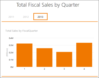
Nearly all data analysis involves browsing and comparing data over dates and time. For example, you may want to sum sales amounts for the past fiscal quarter, and then compare those totals with other quarters, or you may want to calculate a month end closing balance for an account. In each of these cases, you are using dates as a way to group and aggregate sales transactions or balances for a particular period in time.
Power View report
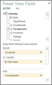
A date table can contain many different representations of dates and time. For example, a date table will often have columns like Fiscal Year, Month, Quarter, or Period that you can select as fields from a Field List when slicing and filtering your data in PivotTables or Power View reports.
Power View Field list
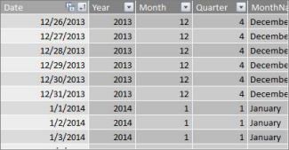
For date columns like Year, Month, and Quarter to include all of the dates within their respective range, the date table must have at least one column with a contiguous set of dates. That is, that column must have one row for every day for each year included in the date table.
For example, if the data you want to browse has dates from February 1st, 2010 through November 30th 2012, and you report on a calendar year, then you will want a date table with at least a date range from January 1st 2010 through December 31st 2012. Every year in your date table must contain all of the days for each year. If you will be regularly refreshing your data with newer data, you might want to run the ending date out by a year or two, so you don’t have to update your date table as time goes by.
Date table with a contiguous set of dates
If you report on a fiscal year, you can create a date table with a contiguous set of dates for each fiscal year. For example, if your fiscal year begins on March 1st, and you have data for fiscal years 2010 up through the current date (for example, in FY 2013), you can create a date table that begins on 3/1/2009 and includes at least every day in each fiscal year through the last date in Fiscal Year 2013.
If you will report on both calendar year and fiscal year, you do not need to create separate date tables. A single date table can include columns for a calendar year, fiscal year, and even a thirteen four-week period calendar. The important thing is your date table contains a contiguous set of dates for all years included.
Adding a date table to the Data Model
There are several ways you can add a date table to your Data Model:
-
Import from a relational database, or other data source.
-
Create a date table in Excel and then copy or link to a new table in Power Pivot.
-
Import from Microsoft Azure Marketplace.
Let’s look at each of these more closely.
Import from a relational database
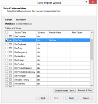
If you import some or all of your data from a data warehouse or other type of relational database, chances are there is already a date table and relationships between it and the rest of data you are importing. The dates and format will likely match the dates in your fact data, and the dates probably begin well in the past and go far out into the future. The date table you want to import may be very large and contain a range of dates beyond what you will need to include in your Data Model. You can use Power Pivot’s Table Import Wizard’s advanced filter features to selectively choose only the dates and the particular columns you really need. This can significantly reduce your workbook’s size and improve performance.
Table Import Wizard
In most cases, you will not need to create any additional columns like Fiscal Year, Week, Month Name, etc. because they will already exist in the imported table. However, in some cases, after you have the date table imported into your Data Model, you might need to create additional date columns, depending on a particular reporting need. Fortunately, this is easy to do using DAX. You will learn more about creating date table fields later. Every environment is different. If you are unsure if your data sources have a related date or calendar table, talk to your database administrator.
Create a date table in Excel
You can create a date table in Excel and then copy it into a new table in the Data Model. This is really quite easy to do and it gives you a lot of flexibility.
When you create a date table in Excel, you begin with a single column with a contiguous range of dates. You can then create additional columns such as Year, Quarter, Month, Fiscal Year, Period, etc. in the Excel worksheet by using Excel formulas, or, after you copy the table into the Data Model, you can create them as calculated columns. Creating additional date columns in Power Pivot is described in the Adding New Date Columns to the Date Table section later in this article.
How to: Create a date table in Excel and copy it into the Data Model
-
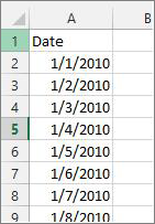
In Excel, in a blank worksheet, in cell A1, type a column header name to identify a range of dates. Typically, this will besomething like Date, DateTime, or DateKey.
-
In cell A2, type a beginning date. For example, 1/1/2010.
-
Click the fill handle and drag it down to a row number that includes an ending date. For example, 12/31/2016.
-
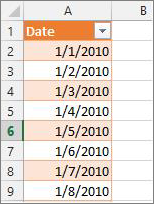
Select all rows in the Date column (including the header name in cell A1).
-
In the Styles group, click Format as Table, and then select a style.
-
In the Format as Table dialog box, click OK.
-
Copy all rows, including the header.
-
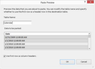
In Power Pivot, on the Home tab, click Paste.
-
In Paste Preview > Table Name type a name such as Date or Calendar. Leave Use first row as column headerschecked, and then click OK.
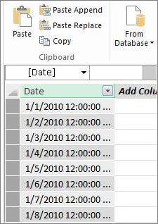
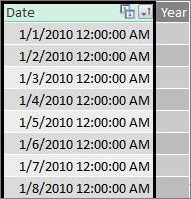
The new date table (named Calendar in this example) in Power Pivot looks like this:
Note: You can also create a linked table by using Add to Data Model. However, this makes your workbook unnecessarily large because the workbook has two versions of the date table; one in Excel and one in Power Pivot..
Note: The name date is a keyword in Power Pivot. If you name the table you create in Power Pivot Date, then you will need to enclose the table name with single quotes in any DAX formulas that reference it in an argument. All of the example images and formulas in this article refer to a date table created in Power Pivot named Calendar.
You now have a date table in your Data Model. You can add new date columns such as Year, Month, etc. by using DAX.
Adding new date columns to the date table
A date table with a single date column that has one row for every day for each year is important for defining all of the dates in a date range. It’s also necessary for creating a relationship between the fact table and the date table. But that single date column with one row for every day is not useful when analyzing by dates in a PivotTable or Power View report. You want your date table to include columns that help you aggregate your data for a range or group of dates. For example, you might want to sum sales amounts by month or quarter, or you may create a measure that calculates year-over-year growth. In each of these cases, your date table needs year, month, or quarter columns that allow you to aggregate your data for that period.
If you imported your date table from a relational data source, it may already include the different types of date columns you want. In some cases, you may want to modify some of those columns or create additional date columns. This is especially true if you create your own date table in Excel and copy it into the Data Model. Fortunately, creating new date columns in Power Pivot is quite easy with Date and Time Functions in DAX.
Tip: If you have not yet worked with DAX, a great place to start learning is with QuickStart: Learn DAX Basics in 30 Minutes on Office.com.
DAX Date and Time Functions
If you’ve ever worked with date and time functions in Excel formulas, then you will likely be familiar with the Date and Time Functions. Though these functions are similar to their counterparts in Excel, there are some important differences:
-
DAX Date and Time functions use a datetime data type.
-
They can take values from a column as an argument.
-
They can be used to return and/or manipulate date values.
These functions are often used when creating custom date columns in a date table, so they are important to understand. We will use a number of these functions to create columns for Year, Quarter, FiscalMonth, and so on.
Note: Date and Time functions in DAX are not the same as Time Intelligence functions. Learn more about Time Intelligence in Power Pivot in Excel.
DAX includes the following Date and Time functions:
There are many other DAX functions you can use in your formulas, too. For example, many of the formulas described here use Math and Trigonometric Functions like MOD and TRUNC, Logical Functions like IF, and Text Functions like FORMAT For more information about other DAX functions, see the Additional Resources section later in this article.
Formula examples for a calendar year
The following examples describe formulas used to create additional columns in a date table named Calendar. One column, named Date, already exists and contains a contiguous range of dates from 1/1/2010 through 12/31/2016.
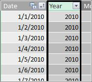
Year
=YEAR([date])
In this formula, the YEAR function returns the year from the value in the Date column. Because the value in the Date column is of datetime data type, the YEAR function knows how to return the year from it.
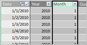
Month
=MONTH([date])
In this formula, much like with the YEAR function, we can simply use the MONTH function to return a month value from the Date column.
Quarter
=INT(([Month]+2)/3)
In this formula, we use the INT function to return a date value as an integer. The argument we specify for the INT function is the value from the Month column, add 2 and then divide that by 3 to get our quarter, 1 thru 4.
Month Name
=FORMAT([date],"mmmm")
In this formula, to get the month name, we use the FORMAT function to convert a numeric value from the Date column to text. We specify the Date column as the first argument, and then the format; we want our month name to show all characters, so we use “mmmm”. Our result looks like this:
If we want to return the month name abbreviated to three letters, we would use “mmm” in the format argument.
Day of Week
=FORMAT([date],"ddd")
In this formula, we use the FORMAT function to get the day name. Because we just want an abbreviated day name, we specify “ddd” in the format argument.

Sample PivotTable
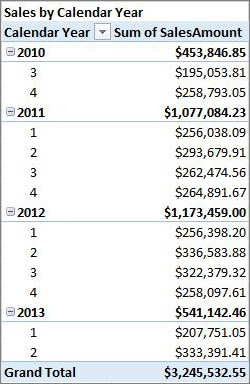
Once you have fields for dates such as Year, Quarter, Month, etc., you can use them in a PivotTable or report. For example, the following image shows the SalesAmount field from the Sales fact table in VALUES, and Year and Quarter from the Calendar dimension table in ROWS. SalesAmount is aggregated for year and quarter context.
Formula examples for a fiscal year
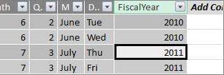
Fiscal Year
=IF([Month]<= 6,[Year],[Year]+1)
In this example, the fiscal year begins on July 1st.
There is no function that can extract a fiscal year from a date value because the start and end dates for a fiscal year are often different from those of a calendar year. To get the fiscal year, we first use an IF function to test if the value for Month is less than or equal to 6. In the second argument, if the value for Month is less than or equal to 6, then return the value from the Year column. If not, then return the value from Year and add 1.
Another way to specify a fiscal year end month value is to create a measure that simply specifies the month. For example, FYE:=6. You can then reference the measure name in place of the month number. For example, =IF([Month]<=[FYE],[Year],[Year]+1). This provides more flexibility when referencing the fiscal year end month in several different formulas.
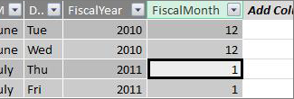
Fiscal Month
=IF([Month]<= 6, 6+[Month], [Month]- 6)
In this formula, we specify if the value for [Month] is less than or equal to 6, then take 6 and add the value from Month, otherwise subtract 6 from the value from [Month].
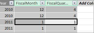
Fiscal Quarter
=INT(([FiscalMonth]+2)/3)
The formula we use for FiscalQuarter is much the same as it was for Quarter in our calendar year. The only difference is we specify [FiscalMonth] instead of [Month].
Holidays or special dates
You may want to include a date column that indicates certain dates are holidays or some other special date. For example, you may want to sum sales totals for New Years day by adding a Holiday field to a PivotTable, as a slicer, or filter. In other cases you may want to exclude those dates from other date columns or in a measure.
Including holidays or special days is quite simple. You can create a table in Excel that has the dates you want to include. You can then copy or use Add to Data Model to add it to the Data Model as a linked table. In most cases, it isn’t necessary to create a relationship between the table and the Calendar table. Any formulas referencing it can use the LOOKUPVALUE function to return values.
Below is an example of a table created in Excel that includes holidays to be added to the date table:
|
Date |
Holiday |
|---|---|
|
1/1/2010 |
New Years |
|
11/25/2010 |
Thanksgiving |
|
12/25/2010 |
Christmas |
|
1/1/2011 |
New Years |
|
11/24/2011 |
Thanksgiving |
|
12/25/2011 |
Christmas |
|
1/1/2012 |
New Years |
|
11/22/2012 |
Thanksgiving |
|
12/25/2012 |
Christmas |
|
1/1/2013 |
New Years |
|
11/28/2013 |
Thanksgiving |
|
12/25/2013 |
Christmas |
|
11/27/2014 |
Thanksgiving |
|
12/25/2014 |
Christmas |
|
1/1/2014 |
New Years |
|
11/27/2014 |
Thanksgiving |
|
12/25/2014 |
Christmas |
|
1/1/2015 |
New Years |
|
11/26/2014 |
Thanksgiving |
|
12/25/2015 |
Christmas |
|
1/1/2016 |
New Years |
|
11/24/2016 |
Thanksgiving |
|
12/25/2016 |
Christmas |
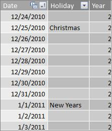
In the date table, we create a column named Holiday and use a formula like this:
=LOOKUPVALUE(Holidays[Holiday],Holidays[date],Calendar[date])
Let’s look at this formula more carefully.
We use the LOOKUPVALUE function to get values from the Holiday column in the Holidays table. In the first argument, we specify the column where our result value will be. We specify the Holiday column in the Holidays table because that is the value we want returned.
=LOOKUPVALUE(Holidays[Holiday],Holidays[date],Calendar[date])
We then specify the second argument, the search column that has the dates we want to search for. We specify the Date column in the Holidays table, like this:
=LOOKUPVALUE(Holidays[Holiday],Holidays[date],Calendar[date])
Finally, we specify the column in our Calendar table that has the dates we want to search for in the Holiday table. This of course is the Date column in the Calendar table.
=LOOKUPVALUE(Holidays[Holiday],Holidays[date],Calendar[date])
The Holiday column will return the holiday name for each row that has a date value that matches a date in the Holidays table.
Custom calendar - thirteen four-week periods
Some organizations, like retail or food service, often report on different periods, like thirteen four-week periods. With a thirteen four-week period calendar, each period is 28 days; therefore, each period contains four Mondays, four Tuesdays, four Wednesdays, and so on. Each period contains the same number of days, and typically, holidays will fall within the same period each year. You can choose to start a period on any day of the week. Just like with dates in a calendar or fiscal year, you can use DAX to create additional columns with custom dates.
In the examples below, the first full period starts on the first Sunday of the fiscal year. In this case, the fiscal year begins on 7/1.
Week
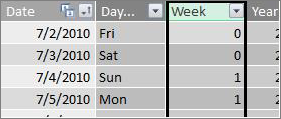
This value gives us the week number starting with the first full week in the fiscal year. In this example, the first full week begins on Sunday, so the first full week in the first fiscal year in the Calendar table actually begins on 7/4/2010 and continues on through the last full week in the Calendar table. While this value itself isn’t all that useful in analysis, it is necessary to calculate for use in other 28 day period formulas.
=INT([date]-40356)/7)
Let’s look at this formula more carefully.
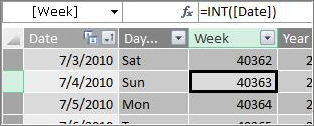
First, we create a formula that returns values from the Date column as an integer, like this:
=INT([date])
We then want to look for the first Sunday in the first fiscal year. We see that it is 7/4/2010.
Now, subtract 40356 (which is the integer for 6/27/2010, the last Sunday from the previous fiscal year) from that value to get the number of days since the start of days in our Calendar table, like this:
=INT([date]-40356)
Then divide the result by 7 (days in a week), like this:
=INT(([date]-40356)/7)
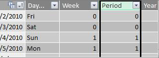
The result looks like this:
Period
The period in this custom calendar contains 28 days and it will always begin on a Sunday. This column will return the number of the period beginning with the first Sunday in the first fiscal year.
=INT(([Week]+3)/4)
Let’s look at this formula more carefully.
First, we create a formula that returns a value from the Week column as an integer, like this:
=INT([Week])
Then add 3 to that value, like this:
=INT([Week]+3)
Then divide the result by 4, like this:
=INT(([Week]+3)/4)
The result looks like this:
Period Fiscal Year
This value returns the fiscal year for a period.
=INT(([Period]+12)/13)+2008
Let’s look at this formula more carefully.
First, we create a formula that returns a value from Period and adds 12:
= ([Period]+12)
We divide the result by 13, because there are thirteen 28 day periods in the fiscal year:
=(([Period]+12)/13)
We add 2010, because that is the first year in the table:
=(([Period]+12)/13)+2010
Finally we use the INT function to remove any fraction of the result, and return a whole number, when divided by 13, like this:
=INT(([Period]+12)/13)+2010
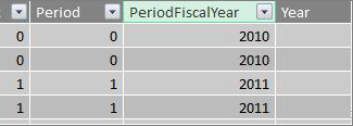
The result looks like this:
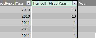
Period in FiscalYear
This value returns the period number, 1 – 13, starting with the first full Period (beginning on Sunday) in each fiscal year.
=IF(MOD([Period],13), MOD([Period],13),13)
This formula is a little more complex, so we will describe it first in a language we better understand. This formula states, divide the value from [Period] by 13 to get a period number (1-13) in the year. If that number is 0, then return 13.
First, we create a formula that returns the remainder of the value from Period by 13. We can use the MOD (Math and Trigonometric functions) like this:
=MOD([Period],13)
This, for the most part, gives us the result we want, except where the value for Period is 0 because those dates don’t fall within the first fiscal year, like in the first five days of our example Calendar date table. We can take care of this with an IF function. In case our result is 0, we return 13, like this:
=IF(MOD([Period],13),MOD([Period],13),13)
The result looks like this:
Sample PivotTable
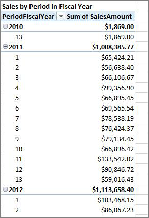
The image below shows a PivotTable with the SalesAmount field from the Sales fact table in VALUES, and PeriodFiscalYear and PeriodInFiscalYear fields from the Calendar date dimension table in ROWS. SalesAmount is aggregated for the context by fiscal year and 28-day period in the fiscal year.
Relationships
After you’ve created a date table in your Data Model, to begin browsing your data in PivotTables and reports, and to aggregate data based on the columns in your date dimension table, you need to create a relationship between the fact table with your transaction data and the date table.
Because you need to create a relationship based on dates, you will want to make sure you create that relationship between columns whose values are of the datetime (Date) data type.
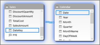
For every date value in the fact table, the related lookup column in the date table must contain matching values. For example, a row (transaction record) in the Sales fact table with a value of 8/15/2012 12:00 AM in the DateKey column must have a corresponding value in the related Date column in the date (named Calendar) table. This is one of the most important reasons you want your date column in the date table to contain a contiguous range of dates that includes any possible date in your fact table.
Note: While the date column in each table must be of the same data type (Date), the format of each column does not matter..
Note: If Power Pivot won’t let you create relationships between the two tables, the date fields may not store the date and time to the same level of precision. Depending on the column formatting, the values may look the same, but be stored differently. Read more about working with time.
Note: Avoid using integer surrogate keys in relationships. When you import data from a relational data source, often date and time columns are represented by a surrogate key, which is an integer column used to represent a unique date. In Power Pivot, you should avoid creating relationships by using integer date/time keys, and instead, use columns that contain unique values with a date data type. Although the use of surrogate keys is considered a best practice in traditional data warehouses, the integer keys are not needed in Power Pivot and can make it difficult to group values in PivotTables by different date periods.
If you get a Type mismatch error when trying to create a relationship, it’s likely because the column in the fact table is not of Date data type. This can happen when Power Pivot cannot automatically convert a non-date (usually a text data type) to a date data type. You can still use the column in your fact table, but you will have to convert the data with a DAX formula in a new calculated column. See Converting text data type dates to a date data type later in the appendix.
Multiple relationships
In some cases, it may be necessary to create multiple relationships or create multiple date tables. For example, if there are multiple date fields in the Sales fact table, such as DateKey, ShipDate, and ReturnDate, they can all have relationships to the Date field in the Calendar date table, but only one of those can be an active relationship. In this case, because DateKey represents the date of the transaction, and therefore the most important date, this would best serve as the active relationship. The others have inactive relationships.
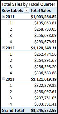
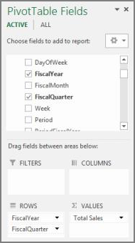
The following PivotTable calculates total sales by Fiscal Year and Fiscal Quarter. A measure named Total Sales, with the formula Total Sales:=SUM([SalesAmount]), is placed in VALUES, and FiscalYear and FiscalQuarter fields from the Calendar date table are placed in ROWS.
This straight-forward PivotTable works correctly because we want to sum our total sales by the transactiondate in DateKey. Our Total Sales measure uses the dates in DateKey and is summed by fiscal year and fiscal quarter because there is a relationship between DateKey in the Sales table and the Date column in the Calendar date table.
Inactive relationships
But, what if we wanted to sum our total sales not by transaction date, but by ship date? We need a relationship between the ShipDate column in the Sales table and the Date column in the Calendar table. If we don’t create that relationship, our aggregations are always based on the transaction date. However, we can have multiple relationships, even though only one can be active, and because transaction date is the most important, it gets the active relationship with the Calendar table.
In this case, ShipDate has an inactive relationship, so any measure formula created to aggregate data based on ship dates must specify the inactive relationship by using the USERELATIONSHIP function.
For example, because there is an inactive relationship between the ShipDate column in the Sales table and the Date column in the Calendar table, we can create a measure that sums total sales by ship date. We use a formula like this to specify the relationship to use:
Total Sales by Ship Date:=CALCULATE(SUM(Sales[SalesAmount]), USERELATIONSHIP(Sales[ShipDate], Calendar[Date]))
This formula simply states: Calculate a sum for SalesAmount, but filter by using the relationship between the ShipDate column in the Sales table and the Date column in the Calendar table.
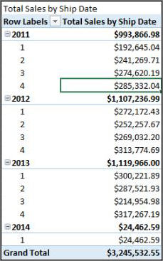
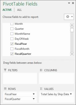
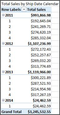
Now, if we create a PivotTable and put Total Sales by Ship Date measure in VALUES, and Fiscal Year and Fiscal Quarter on ROWS, we see the same Grand Total, but all other sum amounts for fiscal year and fiscal quarter are different because they are based on the ship date and not the transaction date.
Using inactive relationships allows you to use only one date table, but it does require that any measures (like Total Sales by Ship Date), reference the inactive relationship in its formula. There is another alternative, that is, use multiple date tables.
Multiple date tables
Another way to work with multiple date columns in your fact table is to create multiple date tables, and create separate active relationships between them. Let’s look at our Sales table example again. We have three columns with dates we might want to aggregate data on:
-
A DateKey with the date of sale for each transaction.
-
A ShipDate – with the date and time when the items sold were shipped to the customer.
-
A ReturnDate – with the date and time when one or more item returned was received.
Remember, the DateKey field with the transaction date is most important. We will do most of our aggregations based on these dates, so we will most certainly want a relationship between it and the Date column in the Calendar table. If we don’t want to create inactive relationships between ShipDate and ReturnDate and the Date field in the Calendar table, thus requiring special measure formulas, we can create additional date tables for ship date and return date. We can then create active relationships between them.
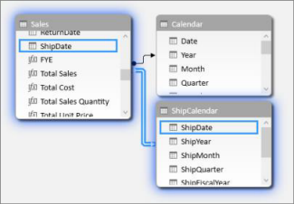
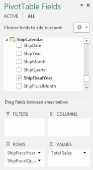
In this example, we’ve created another date table named ShipCalendar. This, of course, also means creating additional date columns, and because these date columns are in a different date table, we want to name them in way that differentiates them from the same columns in the Calendar table. For example, we’ve created columns named ShipYear, ShipMonth, ShipQuarter, and so on.
If we create our PivotTable and put our Total Sales measure in VALUES, and ShipFiscalYear and ShipFiscalQuarter on ROWS, we see the same results that we saw when we created an inactive relationship and a special Total Sales by Ship Date calculated field.
Each of these approaches requires careful consideration. When using multiple relationships with a single date table, you may have to create special measures that transit inactive relationships by using the USERELATIONSHIP function. On the other hand, creating multiple date tables can be confusing in a Field List, and because you have more tables in the Data Model, it will require more memory. Experiment with what works best for you.
Date Table property
The Date Table property sets metadata necessary for Time-Intelligence functions such as TOTALYTD, PREVIOUSMONTH, and DATESBETWEEN to work correctly. When a calculation is run using one of these functions, Power Pivot’s formula engine knows where to go to get the dates it needs.
Warning: If this property is not set, measures using DAX Time-Intelligence functions may not return correct results.
When you set the Date Table property, you specify a date table and a date column of the Date (datetime) data type in it.
How to: Set the Date Table property
-
In the PowerPivot window, select the Calendar table.
-
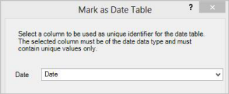
On the Design tab, click Mark as date Table.
-
In the Mark as Date Table dialog box, select a column with unique values and the Date data type.
Working with time
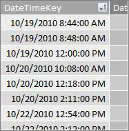
All date values with a Date data type in Excel or SQL Server are actually a number. Included in that number are digits that refer to a time. In many cases, that time for each and every row is midnight. For example, if a DateTimeKey field in a Sales fact table has values like 10/19/2010 12:00:00 AM, this means that the values are to the day level of precision. If the DateTimeKey field values have a time included, for example, 10/19/2010 8:44:00 AM, this means that the values are to the minute level of precision. Values could also be to the hour level precision, or even seconds level of precision. The level of precision in the time value will have a significant impact on how you create your date table and the relationships between it and your fact table.
You need to determine if you will aggregate your data to a day level of precision or to a time level of precision. In other words, you might want to use columns in your date table such as Morning, Afternoon, or Hour as time date fields in a PivotTable’s Row, Column, or Filter areas.
Note: Days are the smallest unit of time that DAX Time Intelligence functions can work with. If you do not need to work with time values, you should reduce the precision of your data to use days as the minimum unit.
If you intend to aggregate your data to the time level, then your date table will need a date column with the time included. In-fact, it will need a date column with one row for every hour, or maybe even every minute, of every day, for every year in the date range. This is because, to create a relationship between the DateTimeKey column in the fact table and the date column in the date table, you must have matching values. As you can imagine, if you include a lot of years, this can make for a very big date table.
In most cases though, you want to aggregate your data only to the day. In other words, you will use columns like Year, Month, Week, or Day of Week as fields in a PivotTable’s Row, Column, or Filter areas. In this case, the date column in the date table need only contain one row for each day in a year, as we described earlier.
If your date column includes a time level of precision, but you will aggregate only to a day level, to create the relationship between the fact table and the date table, you might have to modify your fact table by creating a new column that truncates the values in the date column to a day value. In other words, convert a value like 10/19/2010 8:44:00AM to 10/19/2010 12:00:00 AM. You can then create the relationship between this new column and the date column in the date table because the values match.
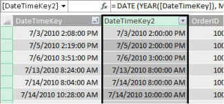
Let’s look at an example. This image shows a DateTimeKey column in the Sales fact table. All of the aggregations for the data in this table need only be to the day level, by using columns in the Calendar date table like Year, Month, Quarter, etc. The time included in the value is not relevant, only the actual date.
Because we don’t need to analyze this data to the time level, we don’t need the Date column in the Calendar date table to include one row for every hour and every minute of every day in each year. So, the Date column in our date table looks like this:
To create a relationship between the DateTimeKey column in the Sales table and the Date column in the Calendar table, we can create a new calculated column in the Sales fact table, and use the TRUNC function to truncate the date and time value in the DateTimeKey column into a date value that matches the values in the Date column in the Calendar table. Our formula looks like this:
=TRUNC([DateTimeKey],0)
This gives us a new column (we named DateKey) with the date from the DateTimeKey column, and a time of 12:00:00 AM for each row:
Now we can create a relationship between this new (DateKey) column and the Date column in the Calendar table.
Similarly, we can create a calculated column in the Sales table that reduces the time precision in the DateTimeKey column to the hour level of precision. In this case, the TRUNC function will not work, but we can still use other DAX Date and Time functions to extract and re-concatenate a new value to an hour level of precision. We can use a formula like this:
= DATE (YEAR([DateTimeKey]), MONTH([DateTimeKey]), DAY([DateTimeKey]) ) + TIME (HOUR([DateTimeKey]), 0, 0)
Our new column looks like this:
Provided our Date column in the date table has values to the hour level of precision, we can then create a relationship between them.
Making dates more usable
Many of the date columns you create in your date table are necessary for other fields, but really aren’t all that useful in analysis. For example, the DateKey field in the Sales table we’ve referred to and shown throughout this article is important because for every transaction, that transaction is recorded as occurring at a particular date and time. But from an analysis and reporting point of view, it is not all that useful because we can’t use it as a row, column, or filter field in a Pivot Table or report.
Similarly, in our example, the Date column in the Calendar table is very useful, critical in-fact, but you cannot use it as a dimension in a PivotTable.
To keep tables and the columns in them as useful as possible, and to make PivotTable or Power View report Field lists easier to navigate, it is important to hide unnecessary columns from client tools. You may also want to hide certain tables as well. The Holidays table shown earlier contains holiday dates that are important for certain columns in the Calendar table, but you can’t use the Date and Holiday columns in the Holidays table themselves as fields in a PivotTable. Here again, to make Field Lists easier to navigate, you can hide the whole Holidays table.
Another important aspect of working with dates is naming conventions. You can name tables and columns in Power Pivot whatever you want. But keep in-mind, especially if you will be sharing your workbook with other users, a good naming convention makes it easier to identify tables and dates, not only in Field Lists, but also in Power Pivot and in DAX formulas.
After you have a date table in your Data Model, you can begin creating measures that will help you get the most out of your data. Some may be as simple as summing sales totals for the current year, and others may be more complex, where you need to filter on a particular range of unique dates. Learn more in Measures in Power Pivot and Time Intelligence Functions.
Appendix
Converting text data type dates to a date data type
In some cases, a fact table with transaction data might contain dates of text data type. That is, a date that appears as 2012-12-04T11:47:09 is in fact not a date at all, or at least not the type of date Power Pivot can understand. It’s really just text that reads like a date. In order to create a relationship between a date column in the fact table, and a date column in a date table, both columns must be of the Date data type.
Typically, when you try to change the data type for a column of dates that are text data type to a date data type, Power Pivot can interpret the dates and convert it to a true date data type automatically. If Power Pivot cannot do a data type conversion, you will get a type mismatch error.
You can, however, still convert the dates into a true date data type. You can create a new calculated column and use a DAX formula to parse the year, month, day, time, etc. from the text strings and then concatenate it back together in a way Power Pivot can read as a true date.
In this example, we’ve imported a fact table named Sales into Power Pivot. It contains a column named DateTime. Values appear like this:
If we look at Data Type in Formatting group Power Pivot’s Home tab, we see that it is Text data type.
We can’t create a relationship between the DateTime column and the Date column in our date table because the data types don’t match. If we try to change the data type to Date, we get a type mismatch error:
In this case, Power Pivot was unable to convert the data type from text to date. We can still use this column, but in order to get it into a true date data type, we need to create a new column that parses the text and re-creates it into a value Power Pivot can make a Date data type.
Remember, from the Working with time section earlier in this article; unless it is necessary your analysis be to a time-of-day level of precision, you should convert dates in your fact table to a day level of precision. With that in-mind, we want the values in our new column to be at the day level of precision (excluding time). We can both convert the values in the DateTime column to a date data type and remove the time level of precision with the following formula:
=DATE(LEFT([DateTime],4), MID([DateTime],6,2), MID([DateTime],9,2))
This gives us a new column (in this case, named Date). Power Pivot even detects the values to be dates and sets the data type automatically to Date.
If we want to preserve the time level of precision, we simply extend the formula to include the hours, minutes, and seconds.
=DATE(LEFT([DateTime],4), MID([DateTime],6,2), MID([DateTime],9,2)) +
TIME(MID([DateTime],12,2), MID([DateTime],15,2), MID([DateTime],18,2))
Now that we have a Date column of the Date data type, we can create a relationship between it and a date column in a date.
Additional resources
QuickStart: Learn DAX Basics in 30 Minutes

