SUMPRODUCT uses cell ranges (or Create an array formula) as its arguments (the parts of the formula that make it work). It multiplies together the items in the arrays, and then sums up the result.
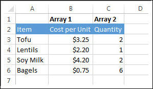
This example is a grocery list, with one array listing the cost for each item, and the other array listing how many items will be purchased.
-
To create the formula, type =SUMPRODUCT(B3:B6,C3:C6) and press Enter.
Each cell in column B is multiplied by its corresponding cell in the same row in column C, and the results are added up. The total amount for the groceries is $21.60.
-
To write a longer formula that gives you the same result, type =B3*C3+B4*C4+B5*C5+B6*C6 and press Enter.
After pressing Enter, the result is the same: $21.60. Cell B3 is multiplied by C3, and its result is added to the result of cell B4 times cell C4 and so on. You can imagine, if you have thousands (or even hundreds) of rows, how much easier using SUMPRODUCT would be.
Notes:
-
The columns or rows (arrays) must be of equal length.
-
If text, instead of a number, is in a cell, it is treated as zero.
Example
If you want to play around with SUMPRODUCT and Create an array formula, here’s an Excel for the web workbook with different data than used in this article.
Copy the example data in the following table, and paste it in cell A1 of a new Excel worksheet. For formulas to show results, select them, press F2, and then press Enter. If you need to, you can adjust the column widths to see all the data.
|
A |
B |
D |
E |
|
|
3 |
4 |
2 |
7 |
|
|
8 |
6 |
6 |
7 |
|
|
1 |
9 |
5 |
3 |
|
|
Formula |
Result |
|||
|
'=SUMPRODUCT(A2:B4,D2:E4) |
=SUMPRODUCT(A2:B4,D2:E4) |
Multiplies all the components of the two arrays (A2:B4 and D2:E4) and then adds the products — that is, 3*2 + 4*7 + 8*6 + 6*7 + 1*5 + 9*3 (156).
For a fuller experience, you can also open this workbook in Excel. Just click the Excel icon on the lower-right corner of the workbook


