Create an array formula

This type of array formula can simplify a worksheet model by replacing several different formulas with a single array formula.

1. Click the cell in which you want to enter the array formula.

2. Enter the formula that you want to use.

   Array formulas use standard formula syntax. They all begin with an equal sign (=), and you can use any of the built-in Excel functions in your array formulas.

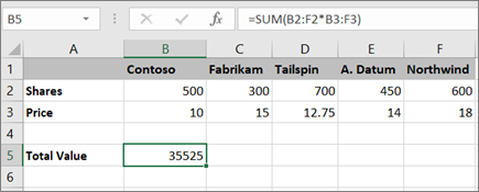
   For example, this formula calculates the total value of an array of stock prices and shares, and places the result in the cell next to "Total Value."

   

   The formula first multiplies the shares (cells B2 – F2) by their prices (cells B3 – F3), and then adds those results to create a grand total of 35,525. This is an example of a single-cell array formula because the formula lives in just one cell.

3. Press Enter (if you have a current Microsoft 365 Subscription); otherwise press Ctrl+Shift+Enter.

   When you press Ctrl+Shift+Enter, Excel automatically inserts the formula between { } (a pair of opening and closing braces).

   Note: If you have a current version of Microsoft 365, then you can simply enter the formula in the top-left-cell of the output range, then press ENTER to confirm the formula as a dynamic array formula. Otherwise, the formula must be entered as a legacy array formula by first selecting the output range, entering the formula in the top-left-cell of the output range, and then pressing CTRL+SHIFT+ENTER to confirm it. Excel inserts curly brackets at the beginning and end of the formula for you. For more information on array formulas, see Guidelines and examples of array formulas.

To calculate multiple results by using an array formula, enter the array into a range of cells that has the exact same number of rows and columns that you’ll use in the array arguments.

1. Select the range of cells in which you want to enter the array formula.

2. Enter the formula that you want to use.

   Array formulas use standard formula syntax. They all begin with an equal sign (=), and you can use any of the built-in Excel functions in your array formulas.

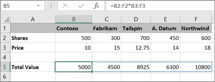
   In the following example, the formula multiples shares by price in each column, and the formula lives in the selected cells in row 5.

   

3. Press Enter (if you have a current Microsoft 365 Subscription); otherwise press Ctrl+Shift+Enter.

   When you press Ctrl+Shift+Enter, Excel automatically inserts the formula between { } (a pair of opening and closing braces).

   Note: If you have a current version of Microsoft 365, then you can simply enter the formula in the top-left-cell of the output range, then press ENTER to confirm the formula as a dynamic array formula. Otherwise, the formula must be entered as a legacy array formula by first selecting the output range, entering the formula in the top-left-cell of the output range, and then pressing CTRL+SHIFT+ENTER to confirm it. Excel inserts curly brackets at the beginning and end of the formula for you. For more information on array formulas, see Guidelines and examples of array formulas.

If you need to include new data in your array formula, see Expand an array formula. You can also try:

• Rules for changing array formulas (they can be finicky)

• Delete an array formula (you press Ctrl+Shift+Enter there, too)

• Use array constants in array formulas (they can be handy)

• Name an array constant (they can make constants easier to use)

If you want to play around with array constants before you try them out with your own data, you can use the sample data here.

The workbook below shows examples of array formulas. To best work with the examples, you should download the workbook to your computer by clicking the Excel icon in the lower-right corner, and then open it in the Excel desktop program.

Copy the table below and paste it into Excel in cell A1. Be sure to select cells E2:E11, enter the formula =C2:C11*D2:D11, and then press Ctrl+Shift+Enter to make it an array formula.

Salesperson	Car Type	Number Sold	Unit Price	Total Sales
Barnhill	Sedan	5	2200	=C2:C11*D2:D11
	Coupe	4	1800
Ingle	Sedan	6	2300
	Coupe	8	1700
Jordan	Sedan	3	2000
	Coupe	1	1600
Pica	Sedan	9	2150
	Coupe	5	1950
Sanchez	Sedan	6	2250
	Coupe	8	2000

Create a multi-cell array formula

1. In the sample workbook, select cells E2 through E11. These cells will contain your results.

You always select the cell or cells that will contain your results before you enter the formula.

And by always, we mean 100-percent of the time.

1. Enter this formula. To enter it in a cell, just start typing (press the equal sign) and the formula appears in the last cell you selected. You can also enter the formula in the formula bar:

   =C2:C11*D2:D11

2. Press Ctrl+Shift+Enter.

Create a single-cell array formula

1. In the sample workbook, click cell B13.

2. Enter this formula using either method from step 2 above:

   =SUM(C2:C11*D2:D11)

3. Press Ctrl+Shift+Enter.

The formula multiplies the values in the cell ranges C2:C11 and D2:D11, then adds the results to calculate a grand total.