#SPILL errors are returned when a formula returns multiple results or a PivotTable range is not blank, and Excel cannot return the results to the grid. For more details on these error types, see the following help topics:
Note: PivotTable #SPILL! is currently available to participants of the Microsoft 365 Insider program.
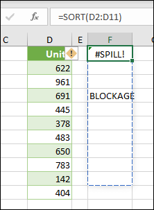
This error occurs when the spill range for a spilled array formula or PivotTable range isn't blank.
Select the cell containing the #SPILL! error to reveal a dashed border that indicates the intended spill range. By selecting the cell containing the #SPILL! error, an error checking alert will appear.
Select the error checking alert and choose the Select Obstructing Cells option to immediately go the obstructing cell(s). You can then clear the error by either deleting, or moving the obstructing cell's entry. As soon as the obstruction is cleared, the array formula will spill or PivotTable will expand as intended.
Excel was unable to determine the size of the spilled array because it's volatile, and resizes between calculation passes. For instance, the following formula will trigger this #SPILL! error:
=SEQUENCE(RANDBETWEEN(1,1000))
Dynamic array resizes may trigger additional calculation passes to ensure the spreadsheet is fully calculated. If the size of the array continues to change during these additional passes and does not stabilize, Excel will resolve the dynamic array as #SPILL!.
This error value is generally associated with the use of RAND, RANDARRAY, and RANDBETWEEN functions. Other volatile functions such as OFFSET, INDIRECT, and TODAY do not return different values on every calculation pass.
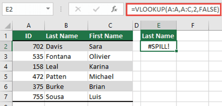
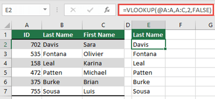
For example, when placed in cell E2 as in the example below, the formula =VLOOKUP(A:A,A:C,2,FALSE) would previously only lookup the ID in cell A2 . However, in dynamic array Excel, the formula will cause a #SPILL! error because Excel will look up the entire column, return 1,048,576 results, and hit the end of the Excel grid.
There are three simple ways to resolve this issue:
|
# |
Approach |
Formula |
|---|---|---|
|
1 |
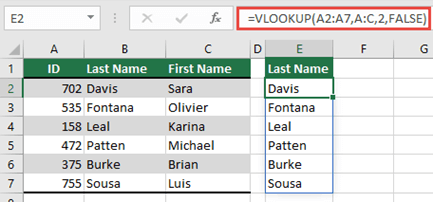
Reference just the lookup values you are interested in. This style of formula will return a dynamic array, but does not work with Excel tables. |
=VLOOKUP(A2:A7,A:C,2,FALSE) |
|
2 |
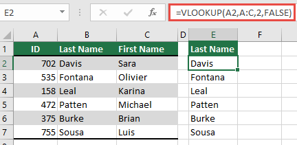
Reference just the value on the same row, and then copy the formula down. This traditional formula style works in tables, but will not return a dynamic array. |
=VLOOKUP(A2,A:C,2,FALSE) |
|
3 |
Request that Excel perform implicit intersection using the @ operator, and then copy the formula down. This style of formula works in tables, but will not return a dynamic array. |
=VLOOKUP(@A:A,A:C,2,FALSE) |
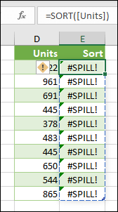
Spilled array formulas aren't supported in Excel tables. Try moving your formula out of the table, or converting the table to a range (select Table Design > Tools > Convert to range).
The spilled array formula you're attempting to enter has caused Excel to run out of memory. Please try referencing a smaller array or range.
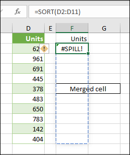
Spilled array formulas cannot spill into merged cells. Please un-merge the cells in question, or move the formula to another range that doesn't intersect with merged cells.
Select the formula to reveal a dashed border that indicates the intended spill range. By selecting the formula, an error checking alert will appear.
You can select the error checking alert, and choose the Select Obstructing Cells option to immediately go the obstructing cell(s). As soon as the merged cells are cleared, the array formula will spill as intended.
Excel doesn't recognize, or can't reconcile the cause of this error. Please make sure your formula contains all the required arguments for your scenario.
Need more help?
See also
You can always ask an expert in the Excel Tech Community or get support in Communities.

