
You can merge (combine) rows from one table into another simply by pasting the data in the first empty cells below the target table. The table will increase in size to include the new rows. If the rows in both tables match up, you can merge the columns of one table with another—by pasting them in the first empty cells to the right of the table. In this case also, the table will increase to accommodate the new columns.
For larger or more complex datasets, you can also combine tables using other tools in Excel.
Merging rows is actually quite simple, but merging columns can be tricky if the rows of one table don't correspond with the rows in the other table. By using a lookup function such as VLOOKUP, you can avoid some of the alignment problems.
Merge two tables using the VLOOKUP function
In the example shown below, you'll see two tables that previously had other names to new names: "Blue" and "Orange." In the Blue table, each row is a line item for an order. So, Order ID 20050 has two items, Order ID 20051 has one item, Order ID 20052 has three items, and so on. We want to merge the Sales ID and Region columns with the Blue table, based on matching values in the Order ID columns of the Orange table.

Order ID values repeat in the Blue table, but Order ID values in the Orange table are unique. If we were to simply copy-and-paste the data from the Orange table, the Sales ID and Region values for the second line item of order 20050 would be off by one row, which would change the values in the new columns in the Blue table.
Here's the data for the Blue table, which you can copy into a blank worksheet. After you paste it into the worksheet, press Ctrl+T to convert it into a table, and then rename the Excel table Blue.
| Order ID | Sale Date | Product ID |
|---|---|---|
| 20050 | 2/2/14 | C6077B |
| 20050 | 2/2/14 | C9250LB |
| 20051 | 2/2/14 | M115A |
| 20052 | 2/3/14 | A760G |
| 20052 | 2/3/14 | E3331 |
| 20052 | 2/3/14 | SP1447 |
| 20053 | 2/3/14 | L88M |
| 20054 | 2/4/14 | S1018MM |
| 20055 | 2/5/14 | C6077B |
| 20056 | 2/6/14 | E3331 |
| 20056 | 2/6/14 | D534X |
Here's the data for the Orange table. Copy it into the same worksheet. After you paste it into the worksheet, press Ctrl+T to convert it into a table, and then rename the table Orange.
| Order ID | Sales ID | Region |
|---|---|---|
| 20050 | 447 | West |
| 20051 | 398 | South |
| 20052 | 1006 | North |
| 20053 | 447 | West |
| 20054 | 885 | East |
| 20055 | 398 | South |
| 20056 | 644 | East |
| 20057 | 1270 | East |
| 20058 | 885 | East |
We need to ensure that the Sales ID and Region values for each order align correctly with each unique order line item. To do this, let's paste the table headings Sales ID and Region into the cells to the right of the Blue table, and use VLOOKUP formulas to get the correct values from the Sales ID and Region columns of the Orange table.
Here's how:
- Copy the headings Sales ID and Region in the Orange table (only those two cells).
- Paste the headings into the cell, to the right of the Product ID heading of the Blue table.
Now, the Blue table is five columns wide, including the new Sales ID and Region columns. - In the Blue table, in the first cell beneath Sales ID, start writing this formula:
=VLOOKUP( - In the Blue table, pick the first cell in the Order ID column, 20050.
The partially completed formula looks like this:
The [@[Order ID]] part means "get the value in this same row from the Order ID column."
Type a comma and select the entire Orange table with your mouse so that "Orange[#All]" is added to the formula. - Type another comma, 2, another comma, and 0—like this: ,2,0
- Press Enter, and the completed formula looks like this:

The Orange[#All] part means "look in all the cells in the Orange table." The 2 means "get the value from the second column," and the 0 means "return the value only if there's an exact match."
Notice that Excel filled the cells down in that column, using the VLOOKUP formula. - Return to step 3, but this time start writing the same formula in the first cell beneath Region.
- In step 6, replace 2 with 3, so the completed formula looks like this:

There's just one difference between this formula and the first formula—the first gets values from column 2 of the Orange table, and the second gets them from column 3.
Now you'll see values in every cell of the new columns in the Blue table. They contain VLOOKUP formulas, but they'll show the values. You'll want to convert the VLOOKUP formulas in those cells to their actual values. - Select all the value cells in the Sales ID column, and press Ctrl+C to copy them.
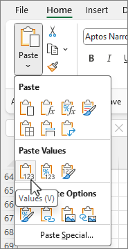
- Select Home > arrow below Paste.

- In the Paste gallery, click Paste Values.
- Select all the value cells in the Region column, copy them, and repeat steps 10 and 11.
Now the VLOOKUP formulas in the two columns have been replaced with the values.
More about tables and VLOOKUP
- Resize a table by adding rows and columns
- Use structured references in Excel table formulas
- VLOOKUP: When and how to use it (training course)
- Get started with Copilot in Excel
Need more help?
You can always ask an expert in the Excel Tech Community or get support in Communities.