To prevent other users from accidentally or deliberately changing, moving, or deleting data in a worksheet, you can lock the cells on your Excel worksheet and then protect the sheet with a password. Say you own the team status report worksheet, where you want team members to add data in specific cells only and not be able to modify anything else. With worksheet protection, you can make only certain parts of the sheet editable and users will not be able to modify data in any other region in the sheet.
Caution: Passwords in Excel for Mac have a 15-character limit. You cannot open a workbook or document that has been password protected in the Windows-based version of Excel or Word if the password is longer than fifteen characters. If you want to open the file in Office for Mac, ask the Windows-based author to adjust the password length. Sheet and workbook element protection should not be confused with workbook-level password security. Element protection cannot protect a workbook from users who have malicious intent. For an additional layer of security, you should help protect your whole workbook file by using a password.
Protect sheet elements
Worksheet protection is a two-step process: the first step is to unlock cells that others can edit, and then you can protect the worksheet with or without a password.
-
Open the sheet that you want to protect.
-
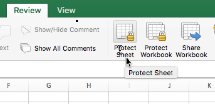
Click Review > Protect Sheet.
-
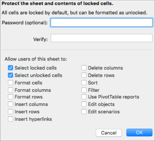
In the Allow users of this sheet to list, select the elements that you want users to be able to change.
Option
Allows users to
Select locked cells
Move the pointer to cells for which the Locked box is checked on the Protection tab of the Format Cells dialog box. By default, users are allowed to select locked cells.
Select unlocked cells
Move the pointer to cells for which the Locked box is unchecked on the Protection tab of the Format Cells dialog box. By default, users can select unlocked cells, and they can press the TAB key to move between the unlocked cells on a protected worksheet.
Format cells
Change any of the options in the Format Cells or Conditional Formatting dialog boxes. If you applied conditional formatting before you protected the worksheet, the formatting continues to change when a user enters a value that satisfies a different condition.
Format columns
Use any of the column formatting commands, including changing column width or hiding columns (Home tab, Cells group, Format button).
Format rows
Use any of the row formatting commands, including changing row height or hiding rows (Home tab, Cells group, Format button).
Insert columns
Insert columns.
Insert rows
Insert rows.
Insert hyperlinks
Insert new hyperlinks, even in unlocked cells.
Delete columns
Delete columns.
Note: If Delete columns is protected and Insert columns is not protected, a user can insert columns but cannot delete them.
Delete rows
Delete rows.
Note: If Delete rows is protected and Insert rows is not protected, a user can insert rows but cannot delete them.
Sort
Use any commands to sort data.
Note: Users can't sort ranges that contain locked cells on a protected worksheet, regardless of this setting.
Filter
Use any commands to filter data.
Use PivotTable reports
Format, change the layout, refresh, or otherwise modify PivotTable reports, or create new reports.
Edit objects
Doing any of the following:
-
Make changes to graphic objects including maps, embedded charts, shapes, text boxes, and controls that you did not unlock before you protected the worksheet. For example, if a worksheet has a button that runs a macro, you can click the button to run the macro, but you cannot delete the button.
-
Make any changes, such as formatting, to an embedded chart. The chart continues to be updated when you change its source data.
-
Add or edit comments.
Edit scenarios
View scenarios that you have hidden, making changes to scenarios that you have prevented changes to, and deleting these scenarios. Users can change the values in the changing cells, if the cells are not protected, and add new scenarios.
-
-
Optional - Enter a password for the sheet, and then retype the password under Verify.
Note: The password is optional. If you do not supply a password, any user can unprotect the sheet and change what was protected. If you do enter a password, make sure that you choose a password that is easy to remember, or write it down and keep it in a safe place. If you lose the password, you cannot access the protected parts on the sheet.
-
Click OK.
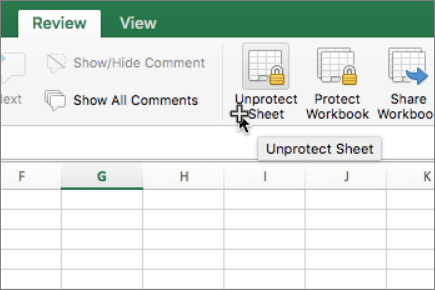
The Protect Sheet option on the ribbon changes to Unprotect Sheet when a sheet is protected.

-
Select the protected sheet.
-
On the Review tab, click Unprotect Sheet.
-
If prompted, enter the password for the protected sheet.
When you unprotect a worksheet, you can unlock graphics, objects, and formulas. See the subsequent section for more information.
When you unprotect a worksheet, you can unlock graphics, objects, ranges, and formulas. See below for more information.
|
To |
Do this |
|---|---|
|
Unlock any cells that you want users to be able to change |
Select each cell or range. On the Format menu, click Cells, click the Protection tab, and then clear the Locked check box. |
|
Unlock any graphic that you want users to be able to change |
Select the graphic, and then on the Format menu, click the command for the type of graphic that you want to unlock: Shape, Text, or Picture. In the navigation pane, click Properties, and then clear the Locked check box. |
|
Unlock any object or control that you want users to be able to change |
Select the object or control, and then on the Format menu, click Format Object or Control. Click the Protection tab, and then clear the Locked check box. Clear the Lock text check box if it is present. |
|
Hide any formulas that you don't want to be visible to users |
Select the cells that contain the formulas. On the Format menu, click Cells, click the Protection tab, and then select the Hidden check box. |
Help us improve Excel
If you have a feature you'd like to request, please send us your feedback to help us prioritize new features in future updates. See How do I give feedback on Microsoft Office for more information.


