

Some of the content in this topic might not apply to all languages.
Conditional formatting makes it easy to highlight certain values or make particular cells easy to identify. This feature changes the appearance of a cell range based on a condition (or criteria). Use conditional formatting to highlight cells that contain values that meet a certain condition. Or format a whole cell range and vary the exact format as the value of each cell varies.
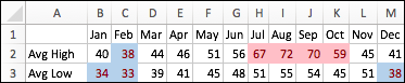
The following example shows temperature information with conditional formatting applied to the top 20% and bottom 20% values:
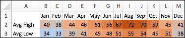
Here's an example with 3-color scale conditional formatting applied:
Apply conditional formatting
Select the range of cells, the table, or the whole sheet where you want to apply conditional formatting.
On the Home tab, select Conditional Formatting.
Do one of the following:
To highlight Do this Values in specific cells. Examples include dates after this week, numbers between 50 and 100, or the bottom 10% of scores. Point to Highlight Cells Rules or Top/Bottom Rules, and then select the appropriate option. The relationship of values in a cell range. Extends a band of color across the cell. Examples include comparisons of prices or populations in the largest cities. Point to Data Bars, and then select the fill that you want. The relationship of values in a cell range. Applies a color scale where the intensity of the cell's color reflects the value's placement toward the top or bottom of the range. An example is sales distributions across regions. Point to Color Scales, and then select the scale that you want. A cell range that contains three to five groups of values, where each group has its own threshold. For example, you might assign a set of three icons to highlight cells that reflect sales below $80,000, sales below $60,000, and sales below $40,000. Or you might assign a 5-point rating system for automobiles and apply a set of five icons. Point to Icon Sets, and then select a set.
More options
Apply conditional formatting to text
- Select the range of cells, the table, or the whole sheet where you want to apply conditional formatting.
- On the Home tab, select Conditional Formatting.
- Point to Highlight Cells Rules, and then select Text that Contains.
- Type the text that you want to highlight, and then select OK.
Create a custom conditional formatting rule
- Select the range of cells, the table, or the whole sheet where you want to apply conditional formatting.
- On the Home tab, click Conditional Formatting.
- Select New Rule.
- Select a style, such as 3-Color Scale, select the conditions that you want, and then select OK.
Format only unique or duplicate cells
- Select the range of cells, the table, or the whole sheet where you want to apply conditional formatting.
- On the Home tab, select Conditional Formatting.
- Point to Highlight Cells Rules, and then select Duplicate Values.
- Next to values in the selected range, select unique or duplicate.
Copy conditional formatting to additional cells
- Select the cell that has the conditional formatting that you want to copy.
- On the Home tab, select Format
 , and then select the cells where you want to copy the conditional formatting.
Find cells that have conditional formatting
If only some part of your sheet has conditional formatting applied, you can quickly locate the cells that are formatted so that you can copy, change, or delete the formatting of those cells.
- Select any cell.
If you want to find only cells with a specific conditional format, start by selecting a cell that has that format. - On the Edit menu, select Find > Go To, and then select Special.
- Select Conditional formats.
If you want to locate only cells with the specific conditional format of the cell that you selected in step 1, select Same.
Clear conditional formatting from a selection
Select the cells that have the conditional formatting that you want to remove.
On the Home tab, select Conditional Formatting.
Point to Clear Rules, and then select the option that you want.
Tip
To remove all conditional formats and all other cell formats for selected cells, on the Edit menu, point to Clear, and then select Formats.
Change a conditional formatting rule
You can customize the default rules for conditional formats to fit your requirements. You can change comparison operators, thresholds, colors, and icons.
- Select a cell in the range that contains the conditional formatting rule that you want to change.
- On the Home tab, select Conditional Formatting.
- Select Manage Rules.
- Select the rule, and then select Edit Rule.
- Make the changes that you want, select OK, and then select OK again.
Delete a conditional formatting rule
You can delete conditional formats that you no longer need.
- Select a cell in the range that contains the conditional formatting rule that you want to change.
- On the Home tab, select Conditional Formatting.
- Select Manage Rules.
- Select the rule, and then select
 .
. - Select OK.