
Learn more about the SUM function.
Quick Sum and the Status Bar
To quickly get the sum of a range of cells, select the range and see the sum displayed in the lower right side of the Excel window.
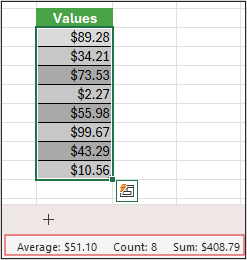
The Status Bar displays information about whatever is currently selected, whether a single cell or multiple cells. Right-click on the Status Bar to see a list of available options. It also displays values for your selected range if you check those attributes.
AutoSum Wizard and Intellisense
The AutoSum Wizard makes it easy to add a SUM formula to your worksheet. Select an empty cell directly above or below the range you want to sum. Then, on the Home or Formulas tab on the Ribbon, select AutoSum > Sum. The AutoSum Wizard automatically detects the range to sum and builds the formula for you. It can also work horizontally if you select a cell to the left or right of the range to sum. It doesn't work on noncontiguous ranges. To learn more, see the subsequent content.
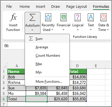
In the AutoSum dialog, you can also select these other common functions:
AutoSum vertically
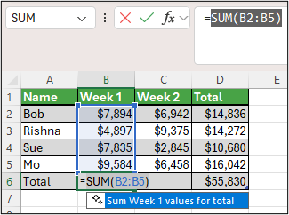
In this example, the AutoSum Wizard automatically detects cells B2:B5 as the range to sum. All you need to do is press Enter to confirm it. To add or exclude cells, hold the appropriate Shift > Arrow key until your selection matches what you want. Then press Enter.
Intellisense function guide
In the image, note the SUM(number1,[number2], …) floating tag beneath the function. This tag is its Intellisense guide. If you select the SUM or function name, it turns into a blue hyperlink that can take you to the Help topic for this function. If you select the individual function elements, their representative pieces in the formula are highlighted. In this case, only B2:B5 is highlighted since there's only one number reference in this formula. The Intellisense tag appears for any function.
AutoSum horizontally
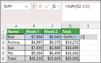
Using SUM with noncontiguous cells
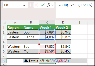
The AutoSum Wizard works best for contiguous ranges. If there's a blank row or column within your sum range, Excel selection stops at the first gap.
In that case, you need to SUM by selection, where you add the individual ranges one by one. In this example, if you had data in cell B4, Excel would generate =SUM(C2:C6) since it recognizes a contiguous range.
You can quickly select multiple noncontiguous ranges by using Ctrl+Left Click. First, enter =SUM(, and then select your different ranges. Excel automatically adds the comma separator between ranges for you. Press Enter when you're done.
Tip
You can use ALT+ = to quickly add the SUM function to a cell. Then all you need to do is select your ranges.
Note
You might notice how Excel highlights the different function ranges by color, and they match within the formula itself. So C2:C3 is one color, and C5:C6 is another. Excel does this for all functions, unless the referenced range is on a different worksheet or in a different workbook. For enhanced accessibility with assistive technology, you can use Named Ranges, like Week1, Week2, and so on, and then reference them in your formula:
=SUM(Week1,Week2)
Using SUM with other functions
You can absolutely use SUM with other functions. Here's an example that creates a monthly average calculation:
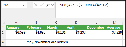
- =SUM(A2:L2)/COUNTA(A2:L2)
This formula takes the SUM of A2:L2 and divides it by the count of nonblank cells in A2:L2 (May through December are blank).
Using SUM across multiple worksheets
Sometimes you need to sum a particular cell on multiple worksheets. It might be tempting to click on each sheet and the cell you want and just use
+to add the cell values, but that method is tedious and can lead to errors.- =Sheet1!A1+Sheet2!A1+Sheet3!A1
You can achieve this result more easily by using a 3D or 3-Dimensional SUM:
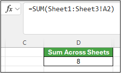
- =SUM(Sheet1:Sheet3!A1)
This formula sums the cell A1 in all sheets from Sheet1 to Sheet3.
This method is particularly helpful in situations where you have a single sheet for each month (January-December) and you need to total them on a summary sheet.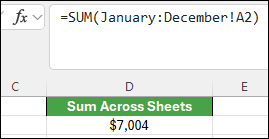
- =SUM(January:December!A2)
This formula sums cell A2 in each sheet from January through December.
Note
If your worksheets have spaces in their names, like "January Sales", then you need to use an apostrophe when referencing the sheet names in a formula. Notice the apostrophe BEFORE the first worksheet name, and again AFTER the last.
- =SUM(‘January Sales:December Sales’!A2)
The 3D method also works with other functions like AVERAGE, MIN, MAX, and more:
- =AVERAGE(Sheet1:Sheet3!A1)
- =MIN(Sheet1:Sheet3!A1)
- =MAX(Sheet1:Sheet3!A1)
Use SUM and other functions to add, subtract, multiply, and divide with Excel
You can easily perform mathematical operations with Excel on their own, and in conjunction with Excel functions like SUM. The following table lists the operators that you can use, along with some related functions. You can input the operators from either the number row on your keyboard, or the 10-key pad if you have one. For instance, Shift+8 enters the asterisk (*) for multiplication.
| Operator | Operation | Examples |
|---|---|---|
| + | Addition | =1+1 =A1+B1 =SUM(A1:A10)+10 =SUM(A1:A10)+B1 |
| - | Subtraction | =1-1 =A1-B1 =SUM(A1:A10)-10 =SUM(A1:A10)-B1 |
| * | Multiplication | =1*1 =A1*B1 =SUM(A1:A10)*10 =SUM(A1:A10)*B1 =PRODUCT(1,1) - PRODUCT function |
| / | Division | =1/1 =A1/B1 =SUM(A1:A10)/10 =SUM(A1:A10)/B1 =QUOTIENT(1,1) - QUOTIENT function |
| ^ | Exponentiation | =1^1 =A1^B1 =SUM(A1:A10)^10 =SUM(A1:A10)^B1 =POWER(1,1) - POWER function |
For more information, see Use Excel as your calculator.
Other Examples
Apply a percentage discount to a range of cells that you summed.
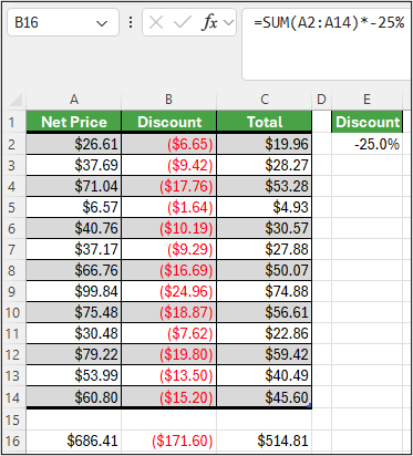
- =SUM(A2:A14)*-25%
This formula gives you 25% of the summed range. However, it hard-codes the 25% in the formula, and it might be hard to find later if you need to change it. Put the 25% in a cell and reference that value instead, where it’s out in the open and easily changed, like this:
- =SUM(A2:A14)*E2
To divide instead of multiply, replace the “*” with “/”: =SUM(A2:A14)/E2
Add or subtract from a SUM
i. You can easily add or subtract from a sum by using + or - like this:- =SUM(A1:A10)+E2
- =SUM(A1:A10)-E2